Rossman Store Sales Prediction
The following project studies a Kaggle use case to predict sales volume for Rossman drug store. An overview of the predictors used, evaluation metrics and leaderboards and be found Here
Rossmann operates over 3,000 drug stores in 7 European countries. Currently, Rossmann store managers are tasked with predicting their daily sales for up to six weeks in advance. Store sales are influenced by many factors, including promotions, competition, school and state holidays, seasonality, and locality. With thousands of individual managers predicting sales based on their unique circumstances, the accuracy of results can be quite varied.
An overview of the training set shows that there are ~1,000,000 rows and 17 columns (1 date, 3 character and 13 numeric), ranging from 2013 till 2015.
Explanatory Data Analysis
Table: Table 1: Data summary
| Name | Piped data |
| Number of rows | 1017209 |
| Number of columns | 17 |
| _______________________ | |
| Column type frequency: | |
| character | 3 |
| Date | 1 |
| numeric | 13 |
| ________________________ | |
| Group variables | None |
Variable type: character
| skim_variable | n_missing | complete_rate | min | max | empty | n_unique | whitespace |
|---|---|---|---|---|---|---|---|
| store_type | 0 | 1.0 | 1 | 1 | 0 | 4 | 0 |
| assortment | 0 | 1.0 | 1 | 1 | 0 | 3 | 0 |
| promo_interval | 508031 | 0.5 | 15 | 16 | 0 | 3 | 0 |
Variable type: Date
| skim_variable | n_missing | complete_rate | min | max | median | n_unique |
|---|---|---|---|---|---|---|
| date | 0 | 1 | 2013-01-01 | 2015-07-31 | 2014-04-02 | 942 |
Variable type: numeric
| skim_variable | n_missing | complete_rate | mean | sd | p0 | p25 | p50 | p75 | p100 | hist |
|---|---|---|---|---|---|---|---|---|---|---|
| store | 0 | 1.00 | 558.43 | 321.91 | 1 | 280 | 558 | 838 | 1115 | ▇▇▇▇▇ |
| day_of_week | 0 | 1.00 | 4.00 | 2.00 | 1 | 2 | 4 | 6 | 7 | ▇▅▅▅▇ |
| sales | 0 | 1.00 | 5773.82 | 3849.93 | 0 | 3727 | 5744 | 7856 | 41551 | ▇▂▁▁▁ |
| open | 0 | 1.00 | 0.83 | 0.38 | 0 | 1 | 1 | 1 | 1 | ▂▁▁▁▇ |
| promo | 0 | 1.00 | 0.38 | 0.49 | 0 | 0 | 0 | 1 | 1 | ▇▁▁▁▅ |
| state_holiday | 31050 | 0.97 | 0.00 | 0.00 | 0 | 0 | 0 | 0 | 0 | ▁▁▇▁▁ |
| school_holiday | 0 | 1.00 | 0.18 | 0.38 | 0 | 0 | 0 | 0 | 1 | ▇▁▁▁▂ |
| competition_distance | 2642 | 1.00 | 5430.09 | 7715.32 | 20 | 710 | 2330 | 6890 | 75860 | ▇▁▁▁▁ |
| competition_open_since_month | 323348 | 0.68 | 7.22 | 3.21 | 1 | 4 | 8 | 10 | 12 | ▅▅▅▆▇ |
| competition_open_since_year | 323348 | 0.68 | 2008.69 | 5.99 | 1900 | 2006 | 2010 | 2013 | 2015 | ▁▁▁▁▇ |
| promo2 | 0 | 1.00 | 0.50 | 0.50 | 0 | 0 | 1 | 1 | 1 | ▇▁▁▁▇ |
| promo2since_week | 508031 | 0.50 | 23.27 | 14.10 | 1 | 13 | 22 | 37 | 50 | ▆▆▂▇▂ |
| promo2since_year | 508031 | 0.50 | 2011.75 | 1.66 | 2009 | 2011 | 2012 | 2013 | 2015 | ▇▇▅▇▆ |
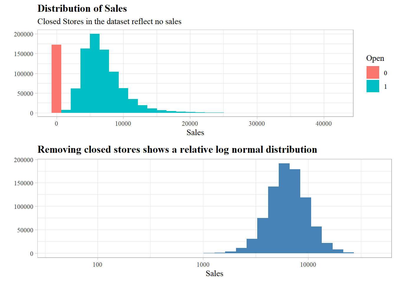
Target Variable
There are closed stores in the dataset which surely have no sales volume, the distribution of sales shows a log normal distribution after filtering for open stores.
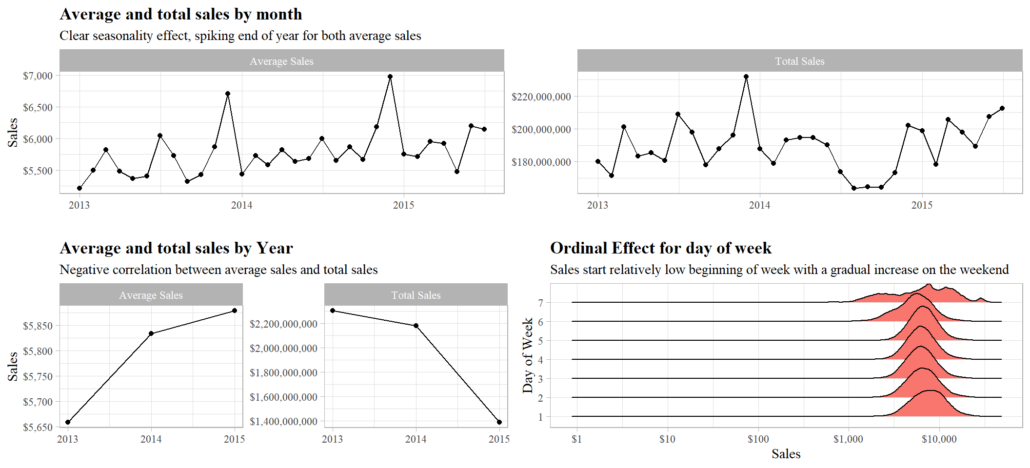
Time series exploration
Fluctation of both average sales and total sales, spiking end of year, effect could be due to natural seasonality or promotions done during that time of year.
Negative correlation, average sale with total sales, could be due to decrease in number of customers, keeping in mind training data is only until Q3 2015, which could be misleading.
Day of week exhibts clear ordinality, as the week starts sales are relativly low as when it ends, with an abnormal distribution on the weekend (day 7)
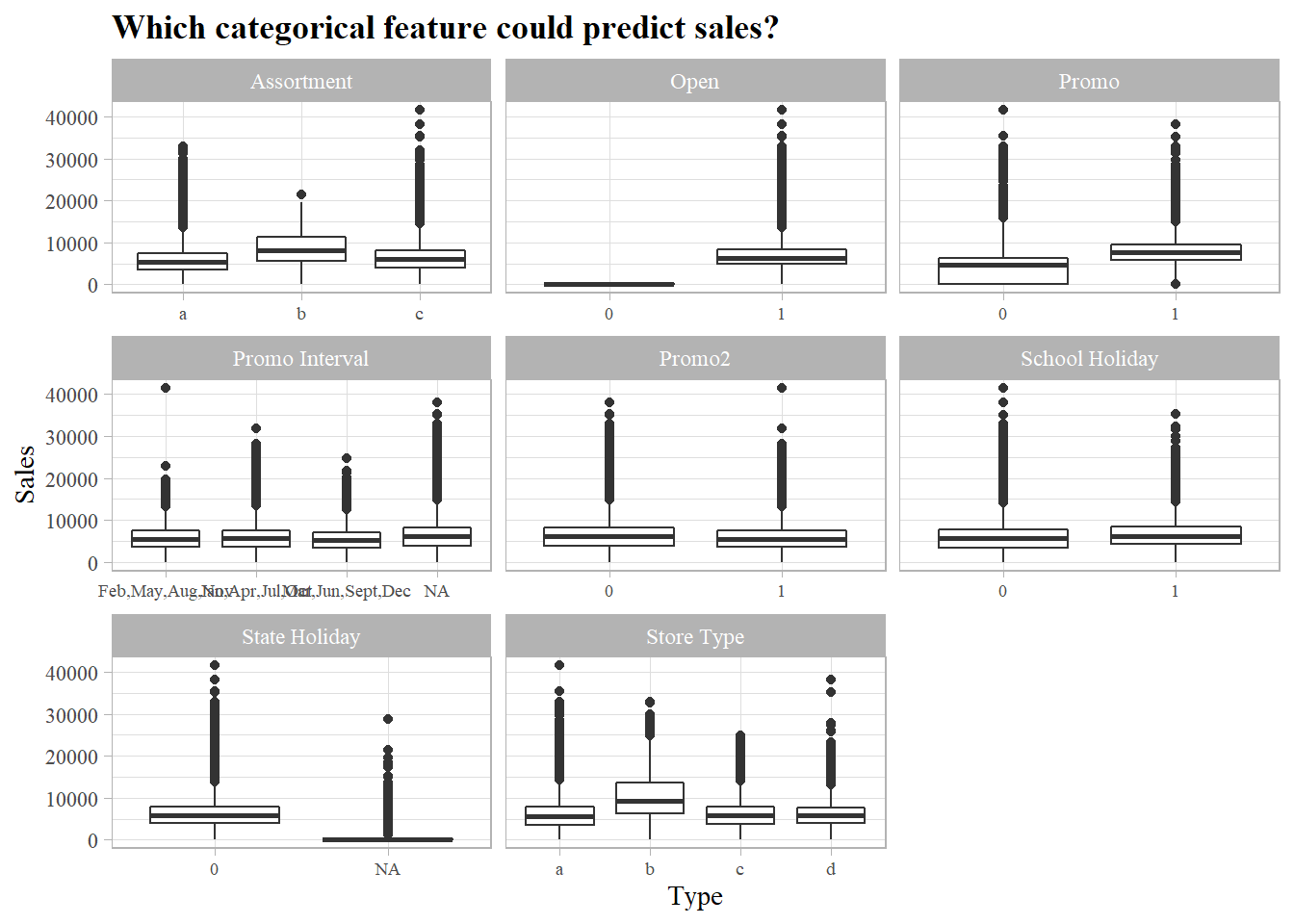
Categorical
Assortment of goods, promotion and store type are good features to use when predicting sales volume.
All closed stores (Open = 0) have 0 sales and any prediction done on closed stores would be neglected (Consider removing from both training and testing sets)
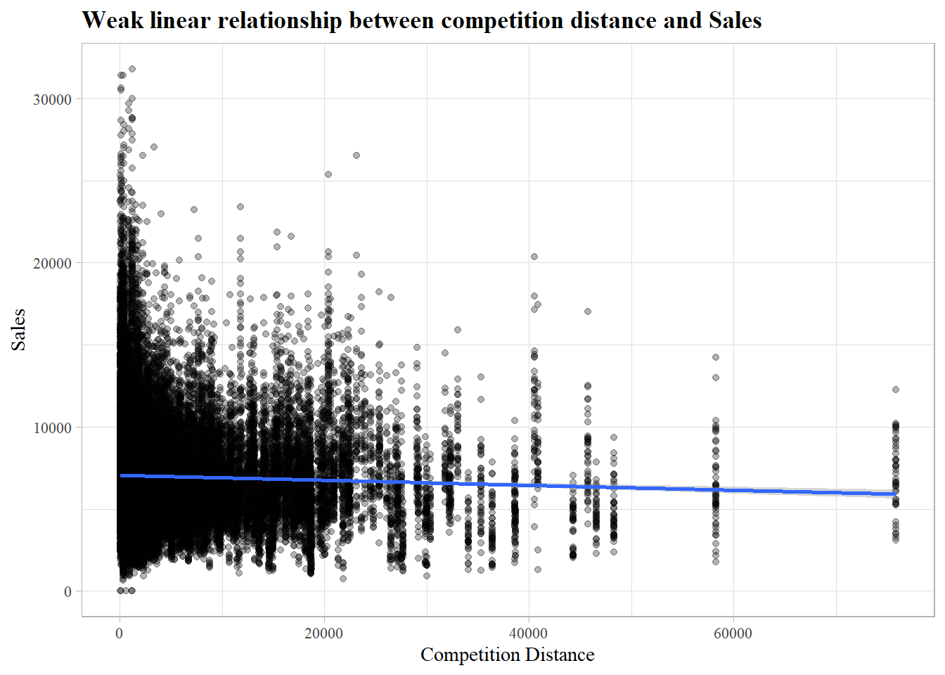
Numeric
One true numeric variable (competition distance), which shows no clear relationship with sales.
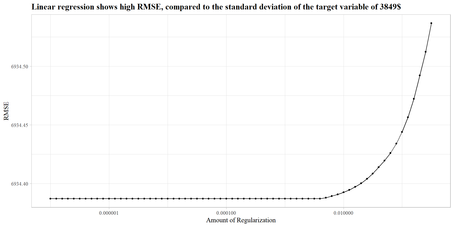
Linear Regression
A 3 fold cross validation linear regression model with regularization (clear not needed) does poorly on the training dataset, as it can not find linear relationships between the target variables and the predictors.
The model scored a RMSPE of 0.38 placing the model in the top 7000
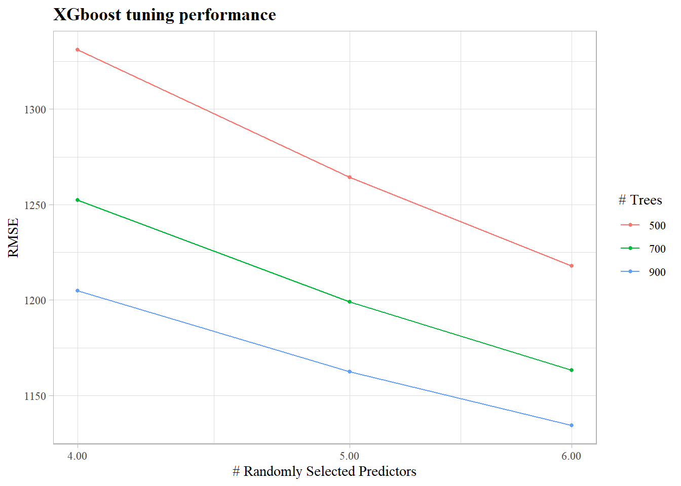
XGBoost
A 3 fold XGBoost model performs much better than the linear model, mtry (number of predictors to use per split) and number of trees were tuned.
The model has not stopped learning even at (mtry = 6,trees = 900) which are the best tuned parameters, which means that the model could be further tuned to provide a lower RMSE
The model scored a RMSPE of 0.166 placing the model in the top 500
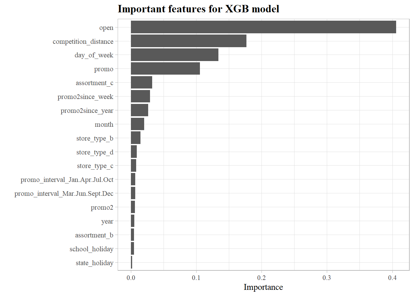
What were the most significant features that the XGBoost model used to predict sales volume?
- Since every store that is closed has 0 sales, the model considers it as an important feature to determine sales which in fact is a redundant feautre
- Competition distance which showed no linear relationship with sales proved to be a very important feature in the XGB model
- Whether a store has a promotional event or not is a good indicator for its sales.
TODO:
- Further parameter tuning
- Remove redundant features and evaluate model performance afterwards
- Ensemble model XGB + Random Forest